Videos
(a)
Construct a
(a)
Answer to Problem 12P
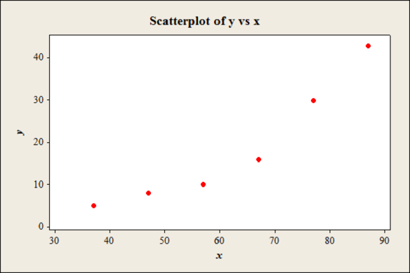
The scatter diagram for data is,
Explanation of Solution
Calculation:
The variable x denotes the age of a licensed driver in years and y denotes the percentage of all fatal accidents due to failure to yield the right-of-way.
Step by step procedure to obtain scatter plot using MINITAB software is given below:
- Choose Graph > Scatterplot.
- Choose Simple. Click OK.
- In Y variables, enter the column of x.
- In X variables, enter the column of y.
- Click OK.
(b)
Verify the values of
(b)
Explanation of Solution
Calculation:
The formula for
In the formula, n is the sample size.
The values are verified in the table below,
| x | y | xy | ||
| 37 | 5 | 1369 | 25 | 185 |
| 47 | 8 | 2209 | 64 | 376 |
| 57 | 10 | 3249 | 100 | 570 |
| 67 | 16 | 4489 | 256 | 1072 |
| 77 | 30 | 5929 | 900 | 2310 |
| 87 | 43 | 7569 | 1849 | 3741 |
Hence, the values are verified.
The number of data pairs are
The value of r is 0.943 this shows that r is not –0.943.
Hence, the value of r is verified as approximately 0.943.
(c)
Find the value of
Find the value of
Find the value of a.
Find the value of b.
Find the equation of the least-squares line.
(c)
Answer to Problem 12P
The value of
The value of
The value of a is –27.768.
The value of b is 0.749.
The equation of the least-squares line is
Explanation of Solution
Calculation:
From part (b), the values are
The value of
Hence, the value of
The value of
Hence, the value of
The value of b is,
Hence, the value of b is 0.749.
The value of a is,
Hence, the value of a is –27.768.
The equation of the least-squares line is,
Hence, the equation of the least-squares line is
(d)
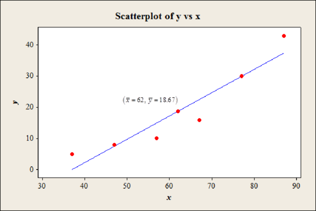
Construct a scatter diagram with least squares line.
Locate the point
(d)
Answer to Problem 12P
The scatter diagram with least squares line with point
Explanation of Solution
Calculation:
In the dataset of failure of yield, also include the point
Step by step procedure to obtain scatter plot using MINITAB software is given below:
- Choose Graph > Scatterplot.
- Choose With regression. Click OK.
- In Y variables, enter the column of x.
- In X variables, enter the column of y.
- Click OK.
(e)
Calculate the value of the coefficient of determination
Mention percentage of the variation in y that can be explained by variation in x.
Mention percentage of the variation in y that cannot be explained by variation in x.
(e)
Answer to Problem 12P
The value of the coefficient of determination
The percentage of the variation in y that can be explained by variation in x is 88.9%.
The percentage of the variation in y that cannot be explained by variation in x is 11.1%.
Explanation of Solution
Calculation:
Coefficient of determination
The coefficient of determination
From part (b), the value of
Hence, the value of the coefficient of determination
About 88.9% of the variation in y (percentage of all fatal accidents due to failure to yield the right-of-way) is explained by x (age of a licensed driver in years). Since the value of
Hence, the percentage of the variation in y that can be explained by variation in x is 92%.
About 11.1%
Hence, the percentage of the variation in y that cannot be explained by variation in x is 11.1%.
(f)
Find the percentage of all fatal accidents due to failing to yield the right-of-way for 70-year-olds.
(f)
Answer to Problem 12P
The percentage of all fatal accidents due to failing to yield the right-of-way for 70-year-olds is 24.662%.
Explanation of Solution
Calculation:
From part (c), the equation of the least-squares line is
Substitute
Hence, the percentage of all fatal accidents due to failing to yield the right-of-way for 70-year-olds is 24.662%.
Want to see more full solutions like this?
Chapter 9 Solutions
Understandable Statistics: Concepts and Methods


- How can one locate mode graphically in case of grouped data?arrow_forwardCan you draw the scatter diagram displaying the data..arrow_forwardSuppose Laura, a facilities manager at a health and wellness company, wants to estimate the difference in the average amount of time that men and women spend at the company's fitness centers each week. Laura randomly selects 15 adult male fitness center members from the membership database and then selects 15 adult female members from the database. Laura gathers data from the past month containing logged time at the fitness center for these members. She plans to use the data to estimate the difference in the time men and women spend per week at the fitness center. The sample statistics are summarized in the table. Population Populationdescription Population mean(unknown) Samplesize Sample mean(min) Sample standarddeviation (min) 11 male μ1 n=15 x¯1=137.7 s=51.7 22 female μ2 n=15 x¯2=114.6 s=34.2 df=24.283 The population standard deviations are unknown and unlikely to be equal, based on the sample data. Laura plans to use the two-sample ?-t-procedures to estimate the…arrow_forward
- Find the correlation coefficient between the “modules studied in the last semester and number of hours spend on reading the books” from your collected data.arrow_forwardThere are two risky shares, where you have calculated the means, and the correlation coefficient of returns between the two shares. Sketch the mean-variance efficient frontier for portfolios of the two shares when the correlation coefficient is +1 and 0 respectively. Explain the shape of the frontier using algebra.arrow_forwardFind the variance of Xarrow_forward
- Describe about the three positive relationships of Scatterplots?arrow_forwardThe mean of the data set {9,5, y, 2, x} is twice the data set {8, x, 4,1,3}. What is (y- x)2?arrow_forwardThe cost of a week long vacation in a city has a mean of 1000 and a variance of 1200. The city imposes a tax which will raise all tourism related costs by 10%. Find the coefficient of variation for the cost of a week long vacation in this city after the tax is imposed.arrow_forward
- Can I have a discussion of this data for my research.arrow_forwardA world wide fast food chain decided to carry out an experiment to assess the influence of advertising expenditure (X) on sales (Y) or vice versa. The table shows, for 8 randomly selected countries, percentage increase in advertisement expenditure (X) and percentage increase in sales (Y) collected. The data presented in the following table are the sums and sum of squares. (use 2 digits after decimal point) EX = 22.5 Ex? = 64.91 5(X-Xbar )? = SSX = 1.63 SY = 135 EY2 = 2595 E(Y-Ybar )? = SSY = 316.88 nx=11 ny=8 Sample mean sales is Sample standard deviation of sales is 90% confidence interval for the population mean sales (hint: assume that sales distributed normally with mean u and variance o?) is [ + 90% confidence interval for the population variance of sales (hint: assume that sales distributed normally with mean u and variance o) is [ toarrow_forwardHomicide and suicide are both intentional means of ending a life. However, the reason for committing a homicide is different from that for suicide and we might expect homicide and suicide rates to be uncorrelated. On the other hand, both can involve some degree of violence, so perhaps we might expect some level of correlation in the rates. The data from 2008–2011 for 26 counties in Ohio are shown in the table. Rates are per 100,000 people. (a) Make a scatterplot that shows how suicide rate can be predicted from homicide rate. There is a weak linear relationship, with correlation ?=0.17. Each of the scatterplots in the choices has a relationship fitted to the plot. Select the plot that corresponds with the correlation of 0.17. (b) Find the least‑squares regression line for predicting suicide rate from homicide rate, ?+?×(homicide). (Enter your answers rounded to three decimal places.) a = b = Explain in words what the slope of the regression line tells us. A) The slope means that for…arrow_forward
 MATLAB: An Introduction with ApplicationsStatisticsISBN:9781119256830Author:Amos GilatPublisher:John Wiley & Sons Inc
 Probability and Statistics for Engineering and th...StatisticsISBN:9781305251809Author:Jay L. DevorePublisher:Cengage Learning
 Statistics for The Behavioral Sciences (MindTap C...StatisticsISBN:9781305504912Author:Frederick J Gravetter, Larry B. WallnauPublisher:Cengage Learning
 Elementary Statistics: Picturing the World (7th E...StatisticsISBN:9780134683416Author:Ron Larson, Betsy FarberPublisher:PEARSON
 The Basic Practice of StatisticsStatisticsISBN:9781319042578Author:David S. Moore, William I. Notz, Michael A. FlignerPublisher:W. H. Freeman
 Introduction to the Practice of StatisticsStatisticsISBN:9781319013387Author:David S. Moore, George P. McCabe, Bruce A. CraigPublisher:W. H. Freeman