Essentials Of Business Analytics
1st Edition
ISBN: 9781285187273
Author: Camm, Jeff.
Publisher: Cengage Learning,
expand_more
expand_more
format_list_bulleted
Videos
Textbook Question
Chapter 5, Problem 14P
The following time series shows the sales of a particular product over the past 12 months.
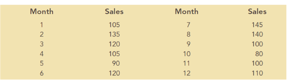
- a. Construct a time series plot. What type of pattern exists in the data?
- b. Use α = 0.3 to compute the exponential smoothing values for the time series.
- c. Use trial and error to find a value of the exponential smoothing coefficient α that results in a relatively small MSE.
Expert Solution & Answer

Trending nowThis is a popular solution!

Chapter 5 Solutions
Essentials Of Business Analytics
Ch. 5 - Consider the following time series data:
Using...Ch. 5 - Refer to the time series data in Problem 1. Using...Ch. 5 - Problems 1 and 2 used different forecasting...Ch. 5 - Consider the following time series data:
Compute...Ch. 5 - Consider the following time series...Ch. 5 - Consider the following time series...Ch. 5 - Prob. 8PCh. 5 - Prob. 9PCh. 5 - Prob. 10PCh. 5 - For the Hawkins Company, the monthly percentages...
Ch. 5 - Corporate triple A bond interest rates for 12...Ch. 5 - The values of Alabama building contracts (in...Ch. 5 - The following time series shows the sales of a...Ch. 5 - Prob. 15PCh. 5 - The following table reports the percentage of...Ch. 5 - Consider the following time series: a. Construct a...Ch. 5 - Consider the following time series:
Construct a...Ch. 5 - The Seneca Children’s Fund (SCF) is a local...Ch. 5 - The president of a small manufacturing firm is...Ch. 5 - Consider the following time series: a. Construct a...Ch. 5 - Consider the following time series...Ch. 5 - The quarterly sales data (number of copies sold)...Ch. 5 - Prob. 25PCh. 5 - South Shore Construction builds permanent docks...Ch. 5 - Hogs & Dawgs is an ice cream parlor on the border...Ch. 5 - Donna Nickles manages a gasoline station on the...Ch. 5 - The Vintage Restaurant, on Captiva Island near...
Knowledge Booster


Learn more about
Need a deep-dive on the concept behind this application? Look no further. Learn more about this topic, statistics and related others by exploring similar questions and additional content below.Similar questions
- What does the y -intercept on the graph of a logistic equation correspond to for a population modeled by that equation?arrow_forwardThe US. import of wine (in hectoliters) for several years is given in Table 5. Determine whether the trend appearslinear. Ifso, and assuming the trend continues, in what year will imports exceed 12,000 hectoliters?arrow_forwardTable 6 shows the population, in thousands, of harbor seals in the Wadden Sea over the years 1997 to 2012. a. Let x represent time in years starting with x=0 for the year 1997. Let y represent the number of seals in thousands. Use logistic regression to fit a model to these data. b. Use the model to predict the seal population for the year 2020. c. To the nearest whole number, what is the limiting value of this model?arrow_forward
- Table 2 shows a recent graduate’s credit card balance each month after graduation. a. Use exponential regression to fit a model to these data. b. If spending continues at this rate, what will the graduate’s credit card debt be one year after graduating?arrow_forwardCable TV The following table shows the number C. in millions, of basic subscribers to cable TV in the indicated year These data are from the Statistical Abstract of the United States. Year 1975 1980 1985 1990 1995 2000 C 9.8 17.5 35.4 50.5 60.6 60.6 a. Use regression to find a logistic model for these data. b. By what annual percentage would you expect the number of cable subscribers to grow in the absence of limiting factors? c. The estimated number of subscribers in 2005 was 65.3million. What light does this shed on the model you found in part a?arrow_forwardEXERCISES The following table gives the life expectancy at birth of females born in the United States in various years from 1970 to 2010. Source: National Center for Health Statistics. Year of Birth Life Expectancy years 1970 74.7 1975 76.6 1980 77.4 1985 78.2 1990 78.8 1995 78.9 2000 79.3 2005 79.9 2010 81.0 Find the life expectancy predicted by your regression equation for each year in the table, and subtract it from the actual value in the second column. This gives you a table of residuals. Plot your residuals as points on a graph.arrow_forward
arrow_back_ios
arrow_forward_ios
Recommended textbooks for you
 Calculus For The Life SciencesCalculusISBN:9780321964038Author:GREENWELL, Raymond N., RITCHEY, Nathan P., Lial, Margaret L.Publisher:Pearson Addison Wesley,
 Functions and Change: A Modeling Approach to Coll...AlgebraISBN:9781337111348Author:Bruce Crauder, Benny Evans, Alan NoellPublisher:Cengage Learning
 Algebra & Trigonometry with Analytic GeometryAlgebraISBN:9781133382119Author:SwokowskiPublisher:Cengage
Calculus For The Life Sciences
Calculus
ISBN:9780321964038
Author:GREENWELL, Raymond N., RITCHEY, Nathan P., Lial, Margaret L.
Publisher:Pearson Addison Wesley,
Functions and Change: A Modeling Approach to Coll...
Algebra
ISBN:9781337111348
Author:Bruce Crauder, Benny Evans, Alan Noell
Publisher:Cengage Learning
Algebra & Trigonometry with Analytic Geometry
Algebra
ISBN:9781133382119
Author:Swokowski
Publisher:Cengage
Time Series Analysis Theory & Uni-variate Forecasting Techniques; Author: Analytics University;https://www.youtube.com/watch?v=_X5q9FYLGxM;License: Standard YouTube License, CC-BY
Operations management 101: Time-series, forecasting introduction; Author: Brandoz Foltz;https://www.youtube.com/watch?v=EaqZP36ool8;License: Standard YouTube License, CC-BY