
(a)
Estimated regression equation.
(a)
Explanation of Solution
The formula for regression equation is:
Run the ordinary least squares method for the given data in excel. The results drawn are as follows:
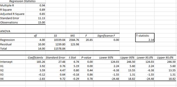
Use the summary output to find the estimated regression equation as follows:
(b)
Economic interpretation of each estimated regression coefficients.
(b)
Explanation of Solution
Interpretation of estimated slope (b) coefficient:
For a given level of total no. of rooms, age and attached garage, an additional 100 ft2 will lead to rise in selling price by 3.92×$1000 = $3,920.
For a given level of size, age and attached garage, an additional room will lead to rise in selling price by 3.59×$1000 = $3,590.
For a given level of size, total no. of rooms and attached garage, an additional year of age will lead to fall in selling price by 0.12×$1000 = $120.
For a given level of size, total no. of rooms and age, an additional garage will lead to fall in selling price by 2.83×$1000 = $2,830.
(c)
Statistical significance of the independent variables at 0.05 level.
(c)
Explanation of Solution
Conduct the t-test to know the statistical significance of the independent variables X1, X2, X3 and X4. The test statistic can be calculated using following formula:
The t-statistic follows t-distribution with n-1 degrees of freedom.
For variable X1, t-test is conducted as follows:
According to the summary output, the t-statistic for X1 variable is equal to 5.19.
At 5% significance level and 15-1= 14 degrees of freedom, the critical value is equal to 2.145.
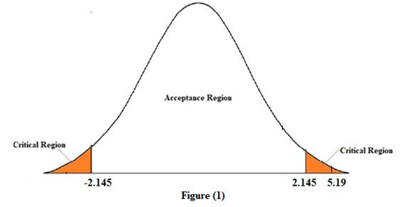
In figure (1), since the calculated t-statistic lies in the critical region. Therefore, we reject the null hypothesis. This means that the variable X1is statistically significant.
For variable X2, t-test is conducted as follows:
According to the summary output, the t-statistic for X2 variable is equal to 0.80.
At 5% significance level and 15-1= 14 degrees of freedom, the critical value is equal to 2.145.
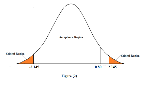
In figure (2), since the calculated t-statistic lies in the acceptance region. Therefore, we accept the null hypothesis. This means that the variable X2is not statistically significant.
For variable X3, t-test is conducted as follows:
According to the summary output, the t-statistic for X3 variable is equal to -0.18.
At 5% significance level and 15-1= 14 degrees of freedom, the critical value is equal to 2.145.
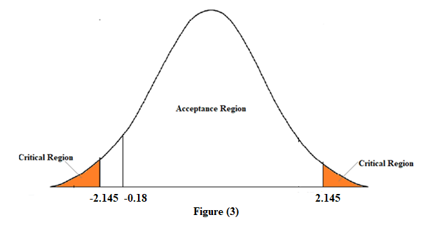
In figure (3), since the calculated t-statistic lies in the acceptance region. Therefore, we accept the null hypothesis. This means that the variable X3is not statistically significant.
For variable X4, t-test is conducted as follows:
According to the summary output, the t-statistic for X4 variable is equal to -0.29.
At 5% significance level and 15-1= 14 degrees of freedom, the critical value is equal to 2.145.
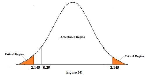
In figure (4), since the calculated t-statistic lies in the acceptance region. Therefore, we accept the null hypothesis. This means that the variable X4is not statistically significant.
(d)
Proportion of total variation in selling price explained by regression model.
(d)
Explanation of Solution
The coefficient of determination measures the proportion of variance predicted by the independent variable in the dependent variable. It is denoted as R2.
According to the summary output, the value of R2 is equal to 0.89. This means that the regression equation predicts 89% of the variance in selling price.
(e)
Overall explanatory power of model by performing F-test at 5 percent level of significance.
(e)
Explanation of Solution
The value of F-statistic is given as 20.85. And the critical value at 0.05 significance level is equal to 0.00.
Since, F-statistic is greater than the critical value. Thus, the overall model is statistically significant.
(f)
95 percent prediction interval for selling price of a 15-year-old house having 1,800 sq. ft., 7 rooms, and an attached garage.
(f)
Explanation of Solution
The confidence interval of a multiple linear regression model can be calculated using following formula:
Here,
y is estimated selling price based on the given values of independent variables
t is critical t value or t-statistic
s.e is multiple standard error of the estimate
The estimated selling price based on the given values of independent variables can be calculated using the estimated regression equation as follows:
According to the regression statistics in the summary output t-statistic and value of multiple standard error of the estimate is equal to 2.14 and 11.13.
Plug the values in the above confidence interval formula as follows:
Thus, an approximate 95% prediction interval for the selling price of a house having an area of a 15-year-old having 1,800 sq. ft., 7 rooms, and an attached garage range from 7291.24 to 7243.60.
Want to see more full solutions like this?
Chapter 4 Solutions
Managerial Economics: Applications, Strategies and Tactics (MindTap Course List)

- Suppose there are 2 quantitative free variables and 1 variable non free category. Non-free variables have 2 categories, namely 1 for the success category and 1 for the fail category. The method used to create models that describe relationships between variables is a binary logistic regression model. Perform parameter recovery for the model. Explain the stage until the alleged value is obtainedarrow_forwardNumerical Answer Only Type Question Enter the numerical value only for the correct answer in the blank box. If a decimal point appears, round it to two decimal places. Assume that the number of visits by a particular customer to a mall located in downtown Toronto is related to the distance from the customer's home. The following regression analysis shows the relationship between the number of times a customer visits(Y)per month and the distance(X, measured in km) from the customer's home to the mall. \[ Y=15-0.5 X \] A customer who lives30 kmaway from the mall will visi______ who lives10 km away. less times than a customerarrow_forwardThe following estimated regression equation relating sales to inventory investment and advertising expenditures was given. ŷ = 21 + 13x1 + 9x2 The data used to develop the model came from a survey of 10 stores; for those data, SST = 19,000 and SSR = 14,630. (a)For the estimated regression equation given, compute R2. R2 = ?? (b)Compute Ra2. (Round your answer to two decimal places.) Ra2 = ?? (c)Does the model appear to explain a large amount of variability in the data? Explain. (For purposes of this exercise, consider an amount large if it is at least 55%. Round your answer to the nearest integer.) The adjusted coefficient of determination shows that (??) % of the variability has been explained by the two independent variables; thus, we conclude that the model does explain a large amount of variability.arrow_forward
- QUESTION 10 Answer questions 10 to 16 based on the regression outputs given in Table 1& 2. Table 1 DATA4-1: Data on single family homes in University City community of San Diego, in 1990. price - sale price in thousands of dollars (Range 199. 9 505) sqft - square feet of living area (Range 1065 - 3000) Table 2 Model 1: OLS, using observations 1-14 Dependent variable: price coefficient std. error t-ratio p-value 52. 3509 0.138750 37. 2855 0.0187329 0. 1857 8. 20e-06 *** const sqft 7. 407 Me dependent var Sun squared resid R-squared F(1, 12) Log-likelihood Schwarz criterion 317. 4929 18273. 57 0. 820522 54. 86051 -70. 08421 145. 4465 Hannan-Quinn S.D. dependent var S.E. of regression Adjusted R-squared P-value (F) Akaike criterion 88. 49816 39. 02304 0. 805565 8. 20e-06 144. 1684 144. 0501 There are observations included in this dataset. It is a. data. O 12; cross-sectional 13; time-series data 14; cross-sectional In this regression model, sale price of a single-family house is the. the…arrow_forwardAn economist believes that price, x, (in dollars) is the biggest factor affecting quantity sold, y. To support his argument, he collected data on price and quantity sold from a sample of 29 stores, selling the same product, and generated the regression output in Excel. The regression equation is reported as y = and the correlation coefficient r = - 0.333. 9.45x + 20.86 What proportion of the variation in quantity sold y can be explained by the variation in price? R² = % Report answer as a percentage accurate to one decimal place.arrow_forwardConduct a regression analysis in Excel using the following data: X Y 12 40 23 50 40 59 33 58 18 45 a) What is the value of b0? Include 1 decimal place in your answer. b) What is the value of b1? Include 2 decimal places in your answer.arrow_forward
- 1. Data were collected on sales of mountain bikes in 30 sporting goods stores. The regression model was y = total sales (thousands of dollars), *₁ = display floor space (square meters), 2 = competitors' advertising expenditures (thousands of dollars), and x3 = advertised price (dollars per unit). A summary of the regression output is below. Variable (nickname) Intercept FloorSpace Competing Ads Price Coefficient 1225.44 11.52 -6.935 -0.1496 (a) Write the fitted regression equation. Round your coefficient Competing Ads to 3 decimal places, coefficient Price to 4 decimal places, and other values to 2 decimal places. (b-1) Put an X in the correct answer circle. The coefficient of FloorSpace says that each additional square foot of floor space... O adds about 11.52 to sales (in thousands of dollars). takes away 11.52 from sales (in thousands of dollars). O adds about 6.935 to sales (in thousands of dollars). takes away 0.1496 from sales (in thousands of dollars). (b-2) Put an X in the…arrow_forwardA home appraisal company would like to develop a regression model that would predict the selling price of a house based on the age of the house in years (X1), the living area of the house in square feet (X2), and the number of bedrooms (X3). The following regression model was chosen using a data set of house statistics: y=88,399554791.3333x231,471.1372x3 The first house from the data set had the following values: Selling price $324,000 Age - 22 years Square Feet 2.000 Bedrooms 3 The residual for this house is 23,558 -41,480 10,216 -16,095 27arrow_forwardInvestigate what factors determine the number of times a person logs into Facebook per week. It is argued that these four factors are important: number of friends, age in years, whether the person is employed, and whether the student has a Twitter account. The function is: FACEBOOK LOGIN=f(FRIENDS,AGE,EMPLOYED,TWITTER) With this functions and variables in mind: Perform necessary tests and analysis to determine the validity of the regression attached in the below table and function provided The tests and analysis must be broken down into two sections namely: tests that are possible with the given regression’s information and tests that should be conducted but are not possible with the given information. For the tests that are possible please conduct them at a 5% significance level and for those that are not possible only mention their names without any further detailsarrow_forward
- Suppose the Sherwin-Williams Company has developed the following multiple regression model, with paint sales Y (x 1,000 gallons) as the dependent variable and promotional expenditures A (x $1,000) and selling price P (dollars per gallon) as the independent variables. Y=α+βaA+βpP+εY=α+βaA+βpP+ε Now suppose that the estimate of the model produces following results: α=344.585α=344.585, ba=0.102ba=0.102, bp=−11.192bp=−11.192, sba=0.173sba=0.173, sbp=4.487sbp=4.487, R2=0.813R2=0.813, and F-statistic=11.361F-statistic=11.361. Note that the sample consists of 10 observations. 1.) According to the estimated model, holding all else constant, a $1,000 increase in promotional expenditures decrease or increase sales by approximately 102,813 or 11,192 gallons. Similarly, a $1 increase in the selling price decrease or increase sales by approximately 813,11,192 or 102 gallons. 2.)Which of the independent variables (if any) appears to be statistically significant (at the 0.05…arrow_forwardConsider the following data regarding students' college GPAs and high school GPAs. The estimated regression equation is Estimated College GPA = 4.59 + (-0.4391) (High School GPA PA). GPAs College GPA High School GPA 2.18 3.25 3.27 4.02 3.20 3.98 3.96 2.26 2.50 3.98 3.32 3.30 Copy Data Step 2 of 3: Compute the mean square error (s) for the model. Round your answer to four decimal places.arrow_forwardSuppose you are the manager of a firm that produces good X in Ghana In order to make informed decision, you engaged an economist to estimate the demand equation for your product. Using data from 30 supermarkets around the country for the month of April, 2021, the estimated linear regression result for your product is shown in the table below: Variable Parameter Estimates Standard error Constant -164.0 20.24 Price of good X (P) Price of good Y (P,) -3.50 1.55 2.50 0.28 Per capita Income () 0.45 0.52 R-squared Adjusted R-squared 0.8672 0.8132 F-statistic 15.6893 a) Suppose the average price of 3 units of good X is GH¢12, price of 2 units of goodY is GH¢60, the per capita income of Ghana is GH¢420. Write down the estimated demand equation for your firm's product and interpret 1. the parameter estimates. Determine the quantity of good X sold. Estimate the own price elasticity of demand and state the type of demand curve 1. 11 your firm has? What would be the effect of a price increase on…arrow_forward
 Managerial Economics: Applications, Strategies an...EconomicsISBN:9781305506381Author:James R. McGuigan, R. Charles Moyer, Frederick H.deB. HarrisPublisher:Cengage Learning