
Concept explainers
Videos
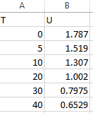
Dynamic viscosity of water
| T | 0 | 5 | 10 | 20 | 30 | 40 |
|
|
1.787 | 1.519 | 1.307 | 1.002 | 0.7975 | 0.6529 |
(a) Plot these data.
(b) Use interpolation to predict
(c) Use polynomial regression to fit a parabola to these data in order to make the same prediction.
(a)
To graph: The given data if
| T | 0 | 5 | 10 | 20 | 30 | 40 |
| 1.787 | 1.519 | 1.307 | 1.002 | 0.7975 | 0.6529 |
Explanation of Solution
Given Information:
The data is,
| T | 0 | 5 | 10 | 20 | 30 | 40 |
| 1.787 | 1.519 | 1.307 | 1.002 | 0.7975 | 0.6529 |
Graph:
The plot can be easily made with the help of excel as shown below,
Step 1. First put the data in the excel as shown below,
Step 2. Now click on insert and then scatter plot.
Thus, the scatter plot is,
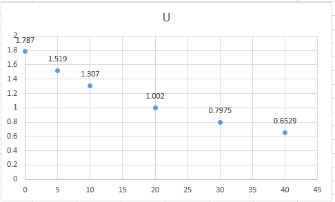
Interpretation:
From the plot, this can be interpreted that the dynamic viscosity of water decreases as the temperature increases.
(b)
To calculate: The value of
| T | 0 | 5 | 10 | 20 | 30 | 40 |
| 1.787 | 1.519 | 1.307 | 1.002 | 0.7975 | 0.6529 |
Answer to Problem 48P
Solution:
The value of
Explanation of Solution
Given Information:
The data is,
| T | 0 | 5 | 10 | 20 | 30 | 40 |
| 1.787 | 1.519 | 1.307 | 1.002 | 0.7975 | 0.6529 |
Formula used:
The zero-order Newton’s interpolation formula:
The first-order Newton’s interpolation formula:
The second- order Newton’s interpolating polynomial is given by,
The n th-order Newton’s interpolating polynomial is given by,
Where,
The first finite divided difference is,
And, the n th finite divided difference is,
Calculation:
To solve for
Assume
First, order the provided value as close to 7.5 as below,
Therefore,
And,
The first divided difference is,
Thus, the first degree polynomial value can be calculated as,
Put
Solve for other values as,
And,
Similarly,
The second divided difference is,
Thus, the second degree polynomial value can be calculated as,
Put
And,
The third divided difference is,
Thus, the third degree polynomial value can be calculated as,
Put this in above equation,
Therefore,
And, the error is calculated as,
Similarly the other dividend can be calculated as shown above,
Therefore, the difference table can be summarized for
| Order | Error | |
| 0 | ||
| 1 | ||
| 2 | ||
| 3 | ||
| 4 | ||
| 5 |
Since the minimum error for order four, therefore, it can be concluded that the value of
(c)
To calculate: The value of
| T | 0 | 5 | 10 | 20 | 30 | 40 |
| 1.787 | 1.519 | 1.307 | 1.002 | 0.7975 | 0.6529 |
Answer to Problem 48P
Solution:
The value of
Explanation of Solution
Given Information:
The data is,
| T | 0 | 5 | 10 | 20 | 30 | 40 |
| 1.787 | 1.519 | 1.307 | 1.002 | 0.7975 | 0.6529 |
Calculation:
This problem can be easily solved with the help of excel as shown below,
Step 1. First put the data in the excel as shown below,
Step 2. Now click on insert and then scatter plot.
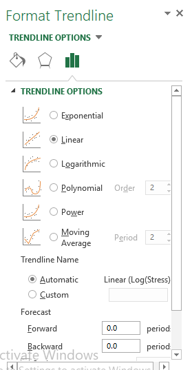
Step 3. Click on layout, Trendline, more trendline options, polynomial and then display equation on chart.
Step 4. Click on display R-squared value on chart as shown below,
Thus, the final plot is shown as below,
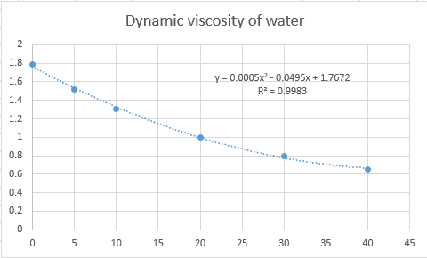
Therefore, the regression plot equation of the data will be,
Put
Hence, the value of
Want to see more full solutions like this?
Chapter 20 Solutions
Numerical Methods for Engineers


- bThe average rate of change of the linear function f(x)=3x+5 between any two points is ________.arrow_forwardUse the total differential to approximate each quantity. Then use a calculator to approximate the quantity, and give the absolute value of the differences in the two results to 4decimal places. (1.922+2.12)13arrow_forwardUse the table of values you made in part 4 of the example to find the limiting value of the average rate of change in velocity.arrow_forward
- The following table provides values of the function f(x,y). However, because of potential; errors in measurement, the functional values may be slightly inaccurately. Using the statistical package included with a graphical calculator or spreadsheet and critical thinking skills, find the function f(x,y)=a+bx+cy that best estimate the table where a, b and c are integers. Hint: Do a linear regression on each column with the value of y fixed and then use these four regression equations to determine the coefficient c. x y 0 1 2 3 0 4.02 7.04 9.98 13.00 1 6.01 9.06 11.98 14.96 2 7.99 10.95 14.02 17.09 3 9.99 13.01 16.01 19.02arrow_forwardFind the intensities of earthquakes whose magnitudes are (a) R=6.0 and (b) R=7.9.arrow_forward
 Calculus For The Life SciencesCalculusISBN:9780321964038Author:GREENWELL, Raymond N., RITCHEY, Nathan P., Lial, Margaret L.Publisher:Pearson Addison Wesley,
 Algebra & Trigonometry with Analytic GeometryAlgebraISBN:9781133382119Author:SwokowskiPublisher:Cengage
 Functions and Change: A Modeling Approach to Coll...AlgebraISBN:9781337111348Author:Bruce Crauder, Benny Evans, Alan NoellPublisher:Cengage Learning
 College AlgebraAlgebraISBN:9781305115545Author:James Stewart, Lothar Redlin, Saleem WatsonPublisher:Cengage Learning
 Algebra and Trigonometry (MindTap Course List)AlgebraISBN:9781305071742Author:James Stewart, Lothar Redlin, Saleem WatsonPublisher:Cengage Learning