
Videos
a.
Test whether the given model is useful or not at the 0.05 level of significance.
a.
Answer to Problem 46E
There is convincing evidence that the given model is useful at the 0.05 level of significance.
Explanation of Solution
Calculation:
It is given that the variable y is absorption,
1.
The model is
2.
Null hypothesis:
That is, there is no useful relationship between y and any of the predictors.
3.
Alternative hypothesis:
That is, there is a useful relationship between y and any of the predictors.
4.
Here, the significance level is
5.
Test statistic:
Here, n is the sample size, and k is the number of variables in the model.
6.
Assumptions:
Since there is no availability of original data to check the assumptions, there is a need to assume that the variables are related to the model, and the random deviation is distributed normally with mean 0 and the fixed standard deviation.
7.
Calculation:
From the MINITAB output, the value of
The value of F-test statistic is calculated as follows:
8.
P-value:
Software procedure:
Step-by-step procedure to find the P-value using the MINITAB software:
- Choose Graph > Probability Distribution Plot choose View Probability > OK.
- From Distribution, choose ‘F’ distribution.
- Enter the Numerator df as 2 and Denominator df as 25.
- Click the Shaded Area tab.
- Choose X Value and Right Tail for the region of the curve to shade.
- Enter the X value as 334.722.
- Click OK.
Output obtained using the MINITAB software is represented as follows:
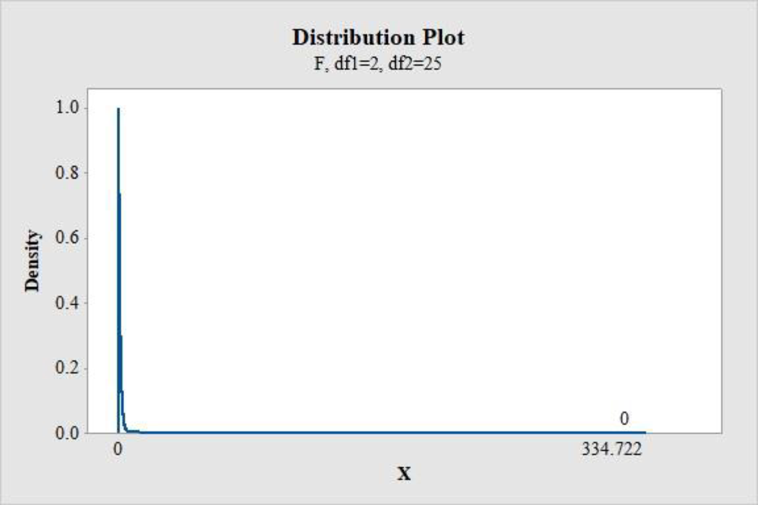
From the MINITAB output, the P-value is 0.
9.
Conclusion:
If the
Therefore, the P-value of 0 is less than the 0.05 level of significance.
Hence, reject the null hypothesis.
Thus, there is convincing evidence that the given model is useful at the 0.05 level of significance.
b.
Calculate a 95% confidence interval for
b.
Answer to Problem 46E
The 95% confidence interval for
Explanation of Solution
Calculation:
Here,
Since there is no availability of original data to check the assumptions, there is a need to assume that the variables are related to the model, and the random deviation is distributed normally with mean 0 and the fixed standard deviation.
The formula for confidence interval for
Where,
Degrees of freedom:
Software procedure:
Step-by-step procedure to find the P-value using the MINITAB software:
- Choose Graph > Probability Distribution Plot choose View Probability > OK.
- From Distribution, choose ‘t’ distribution.
- Enter the Degrees of freedom as 25.
- Click the Shaded Area tab.
- Choose Probability and Both for the region of the curve to shade.
- Enter the Probability value as 0.05.
- Click OK.
Output obtained using the MINITAB software is represented as follows:
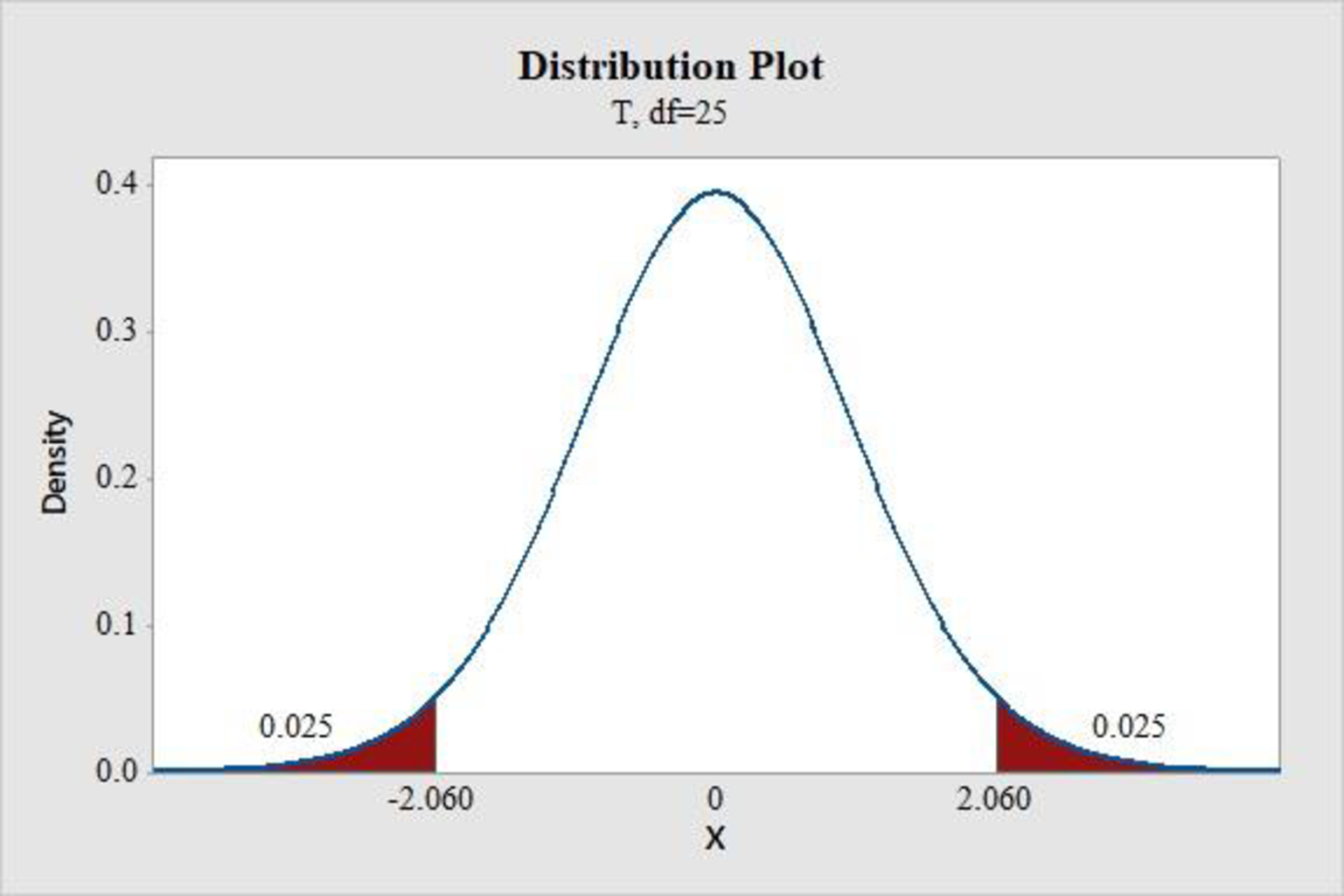
From the MINITAB output, the critical value is 2.060.
From the given MINITAB output, the value of
The confidence interval for mean change in exam score is calculated as follows:
Thus, the 95% confidence interval for
There is 95% confident that the average increase in y is associated with 1-unit increase in starch damage that is between 0.298 and 0.373, when the other predictors are fixed.
c.
- i. Test the hypothesis
H 0 : β 1 = 0 H a : β 1 ≠ 0
- ii. Test the hypothesis
H 0 : β 2 = 0 H a : β 2 ≠ 0
c.
Answer to Problem 46E
It can be concluded that the quadratic term should not be eliminated from the model and simple linear model should not be sufficient.
Explanation of Solution
Calculation:
i.
1.
The predictor
2.
Null hypothesis:
3.
Alternative hypothesis:
4.
Here, the common significance levels are
5.
Test statistic:
Here,
6.
Assumptions:
The random deviations from the values by the population regression equation are distributed normally with mean 0 and fixed standard deviation.
7.
Calculation:
From the MINITAB output, the t test statistic value of
8.
P-value:
From the MINITAB output, the P-value for
9.
Conclusion:
If the
Therefore, the P-value of 0 is less than any common levels of significance, such as 0.05, 0.01, and 0.10.
Hence, reject the null hypothesis.
Thus, there is convincing evidence that the flour protein variable is important and it is
ii.
1.
The predictor
2.
Null hypothesis:
3.
Alternative hypothesis:
4.
Here, the common significance levels are
5.
Test statistic:
Here,
6.
Assumptions:
The random deviations from the values by the population regression equation are distributed normally with mean 0 and fixed standard deviation.
7.
Calculation:
From the MINITAB output, the t test statistic value of
8.
P-value:
From the MINITAB output, the P-value for
9.
Conclusion:
If the
Therefore, the P-value of 0 is less than any common levels of significance, such as 0.05, 0.01, and 0.10.
Hence, reject the null hypothesis.
Thus, there is convincing evidence that the starch damage variable is important and it is
d.
Explain whether both the independent variables are important or not.
d.
Explanation of Solution
From the results of Part (c), there is evidence that the variables of flour protein and starch damage are important.
e.
Calculate a 90% confidence interval and interpret it.
e.
Answer to Problem 46E
The 90% confidence interval is
Explanation of Solution
Calculation:
It is given that the value of
Assume that the exam score is associated with the predictors according to the model. The random deviations from the values by the population regression equation are distributed normally with mean 0 and fixed standard deviation.
The formula for prediction interval for
The value of
Degrees of freedom:
Software procedure:
Step-by-step procedure to find the P-value using the MINITAB software:
- Choose Graph > Probability Distribution Plot choose View Probability > OK.
- From Distribution, choose ‘t’ distribution.
- Enter the Degrees of freedom as 25.
- Click the Shaded Area tab.
- Choose Probability and Both for the region of the curve to shade.
- Enter the Probability value as 0.10.
- Click OK.
Output obtained using the MINITAB software is represented as follows:
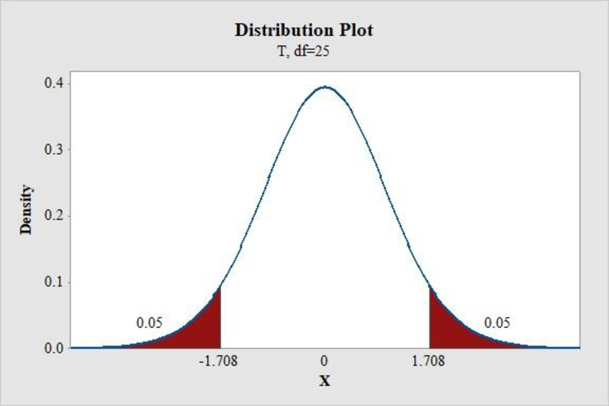
From the MINITAB output, the critical value is 1.708.
The prediction interval for mean y value is calculated as follows:
Thus, the 90% confidence interval is
There is 90% confident that the mean water absorption for wheat with 11.7 flour protein and 57 starch damage is between 54.5084 and 56.2916.
f.
Predict the water absorption for the shipment by 90% interval.
f.
Answer to Problem 46E
The water absorption values for the particular shipment are between 53.3297 and 57.4703 by 90% prediction interval.
Explanation of Solution
Calculation:
It is given that the value of
Assume that the exam score is associated with the predictors according to the model. The random deviations from the values by the population regression equation are distributed normally with mean 0 and fixed standard deviation.
The formula for prediction interval for mean y value is as follows:
From the given MINITAB output, the standard deviation is 1.094.
From Part e., the value of
From the MINITAB output in Part e., the critical value is 1.708.
The prediction interval for water absorption for shipment is calculated as follows:
Thus, the 90% prediction interval is
By prediction at 90% interval, the water absorption values for the particular shipment are between 53.3297 and 57.4703.
Want to see more full solutions like this?
Chapter 14 Solutions
Introduction To Statistics And Data Analysis


- Solve An article in the ASCE Journal of Energy Engineering (1999, Vol. 125, pp.59-75) describes a study of the thermal inertia properties of autoclaved aerated concrete used as a building material. Five samples of the material were tested in a structure, and the average interior temperatures (°C) reported were as follows: 23.01, 22.22, 22.04, 22.62, and 22.59. Test that the average interior temperature is equal to 22.5°C using alpha (a) = 0.05. 1.)This problem is a test on what population parameter? a.Variance/ Standard Deviation b.Mean c.Population Proportion d.None of the above 2.)What is the null and alternative 3 points hypothesis? a.Ho / (theta = 22.5) , Ha: (0 # 22.5) b.Ho / (theta > 22.5) , Ha: (0 # 22.5) c.Ho / (theta < 22.5) , Ha: (theta >= 22.5) d.None of the above 3.)What are the Significance level 3 points and type of test? alpha = 0.05 two-tailed alpha = 0.95 two-tailed alpha = 0.95 one-tailed None of the above 4.)What standardized test statistic will…arrow_forwardExplain the Stationarity in the AR(1) Model?arrow_forwardConsider a simple linear regression model Yi = Bo + B1xi + Ei, i= 1,2, 3 with x; = i/3 for i = 1, 2, 3. Assume that %3| E1 1 -1 0 E = E2 ~ N -1 E3. 3 What is the smallest variance for an unbiased estimate of B1?arrow_forward
- A deficiency of the trace element selenium in the diet can negatively impact growth, immunity, muscle and neuromuscular function, and fertility. The introduction of selenium supplements to dairy cows is justified when pastures have low selenium levels. Authors of a research paper supplied the following data on milk selenium concentration (mg/L) for a sample of cows given a selenium supplement (the treatment group) and a control sample given no supplement, both initially and after a 9-day period. Initial Measurement Treatment Control 11.4 9.1 9.6 8.7 10.1 9.7 8.5 10.8 10.2 10.9 10.6 10.6 11.9 10.1 9.9 12.3 10.7 8.8 10.2 10.4 10.3 10.9 11.4 10.4 9.3 11.6 10.6 10.9 10.9 8.3 After 9 Days Treatment Control 138.3 9.2 104 8.9 96.4 8.9 89 10.1 88 9.6 103.8 8.6 147.3 10.4 97.1 12.4 172.6 9.2 146.3 9.5 99 8.4 122.3 8.8 103 12.5 117.8 9.1 121.5 93 (a) Use the given data for the treatment group to determine if…arrow_forwardA deficiency of the trace element selenium in the diet can negatively impact growth, immunity, muscle and neuromuscular function, and fertility. The introduction of selenium supplements to dairy cows is justified when pastures have low selenium levels. Authors of a research paper supplied the following data on milk selenium concentration (mg/L) for a sample of cows given a selenium supplement (the treatment group) and a control sample given no supplement, both initially and after a 9-day period. Initial Measurement Treatment Control 11.2 9.1 9.6 8.7 10.1 9.7 8.5 10.8 10.3 10.9 10.6 10.6 11.7 10.1 9.7 12.3 10.8 8.8 10.3 10.4 10.4 10.9 11.2 10.4 9.4 11.6 10.6 10.9 10.7 8.4 After 9 Days Treatment Control 138.3 9.3 104 8.7 96.4 8.7 89 10.1 88 9.6 103.8 8.6 147.3 10.2 97.1 12.2 172.6 9.3 146.3 9.5 99 8.2 122.3 8.9 103 12.5 117.8 9.1 121.5 93 (a) Use the given data for the treatment group to determine if there…arrow_forwardA deficiency of the trace element selenium in the diet can negatively impact growth, immunity, muscle and neuromuscular function, and fertility. The introduction of selenium supplements to dairy cows is justified when pastures have low selenium levels. Authors of a research paper supplied the following data on milk selenium concentration (mg/L) for a sample of cows given a selenium supplement (the treatment group) and a control sample given no supplement, both initially and after a 9-day period. Initial Measurement Treatment Control 11.3 9.1 9.7 8.7 10.1 9.7 8.5 10.8 10.4 10.9 10.7 10.6 11.8 10.1 9.8 12.3 10.6 8.8 10.4 10.4 10.2 10.9 11.3 10.4 9.2 11.6 10.7 10.9 10.8 8.2 After 9 Days Treatment Control 138.3 9.4 104 8.8 96.4 8.8 89 10.1 88 9.7 103.8 8.7 147.3 10.3 97.1 12.3 172.6 9.4 146.3 9.5 99 8.3 122.3 8.9 103 12.5 117.8 9.1 121.5 93 (a) Use the given data for the treatment group to determine if…arrow_forward
- A statistical program is recommended.A highway department is studying the relationship between traffic flow and speed. The following model has been hypothesized:y = 0 + 1x + wherey traffic flow in vehicles per hourx = vehicle speed in miles per hour.The following data were collected during rush hour for six highways leading out of the city.Traffic Flow(y)Vehicle Speed(x )1,247351,320401,218301, 327451,341501, 11325(a) Develop an estimated regression equation for the data. (Round bo to one decimal place and b1 to two decimal places.) =arrow_forwardIs it possible to get the following from a set of experimental data: (a) r23 = 0.8, r13 = - 0.5, r12 = 0.6 %3D %3D %3D (b) r23 = 0.7, r13 = - 0.4, r12 = 0.6 %3D %3D %3Darrow_forwardDistilled H2O 20 19.95 20.15 20.1 20.08 19.96 19.96 20.14 20.04 19.95 19.99 20.03 19.95 20.07 20 19.95 20.05 20.05 20.06 19.93 Petro 19.84 20.08 19.82 19.91 20.06 19.96 20.09 19.91 20.03 19.86 19.99 19.89 19.81 19.95 20.08 19.95 19.92 20.06 19.95 19.82 NaCl 20 19.99 20.07 20 19.83 20.03 19.93 20.04 19.97 19.93 20.02 20.02 19.87 19.95 19.91 20 20.09 19.98 19.81 20.05 MgCl 19.88 19.86 19.8 19.95 19.83 19.93 19.9 19.95 19.98 19.86 20.1 19.79 19.83 20.07 19.8 19.78 20.02 20.07 19.92 20.08 NaCl + MgCl 19.93 19.84 19.9 19.82 19.93 19.82 19.88 19.9 19.82 19.83 19.97 19.81 19.88 19.88 19.83 19.81 19.7 19.8 19.82 19.83arrow_forward
- Wrinkle recovery angle and tensile strength are the two most important characteristics for evaluating the performance of crosslinked cotton fabric. An increase in the degree of crosslinking, as determined by ester carboxyl band absorbance, improves the wrinkle resistance of the fabric (at the expense of reducing mechanical strength). The accompanying data on x = absorbance and y = wrinkle resistance angle was read from a graph in the paper "Predicting the Performance of Durable Press Finished Cotton Fabric with Infrared Spectroscopy".t 半 0.115 0.126 0.183 0.246 0.282 0.344 0.355 0.452 0.491 0.554 0.651 334 342 355 363 365 372 381 392 400 412 420 Here is regression output from Minitab: Predictor Coef SE Coef P Constant 321.878 2.483 129.64 0.000 absorb 156.711 6.464 24.24 0.000 S = 3.60498 R-Sq = 98.5% R-Są (adj) - 98.3% SOURCE DF MS F P Regression 1 7639.0 7639.0 587.81 0.000 Residual Error 9 117.0 13.0 Total 10 7756.0 (a) Does the simple linear regression model appear to be…arrow_forwardWrinkle recovery angle and tensile strength are the two most important characteristics for evaluating the performance of crosslinked cotton fabric. An increase in the degree of crosslinking, as determined by ester carboxyl band absorbance, improves the wrinkle resistance of the fabric (at the expense of reducing mechanical strength). The accompanying data on x = absorbance and y = wrinkle resistance angle was read from a graph in the paper "Predicting the Performance of Durable Press Finished Cotton Fabric with Infrared Spectroscopy".† x 0.115 0.126 0.183 0.246 0.282 0.344 0.355 0.452 0.491 0.554 0.651 y 334 342 355 363 365 372 381 392 400 412 420 Here is regression output from Minitab: Predictor Constant absorb S = 3.60498 Coef 321.878 156.711 SOURCE Regression Residual Error Total SE Coef 2.483 6.464 R-Sq = 98.5% DF 1 9 10 SS 7639.0 117.0 7756.0 T 129.64 24.24 0.000 0.000 R-Sq (adj) = 98.3% MS 7639.0 13.0 F P 587.81 (a) Does the simple linear regression model appear to be…arrow_forwardQuestion 3. a) A Biologist is comparing intervals (m seconds) between the matting calls of a certain species of tree frog and the surrounding temperature (t degree Celsius). The following results were obtained: t 8 13 14 15 15 20 25 30 6.5 4.5 4 3 2 1 1. Fit the regression line in the form m = a + bt. 2. Interpret your estimates. 3. Use your regression line interval between matting calls when the surrounding temperature is 10 degrees. (6 marks) estimate the timearrow_forward
 Calculus For The Life SciencesCalculusISBN:9780321964038Author:GREENWELL, Raymond N., RITCHEY, Nathan P., Lial, Margaret L.Publisher:Pearson Addison Wesley,