
Videos
a.
Find the regression line for the variables fracture toughness
Test whether there is enough evidence to conclude that the predictor variable mode-mixity angle is useful for predicting the value of the response variable fracture toughness.
a.
Answer to Problem 76SE
The regression line for the variables fracture toughness
There is sufficient evidence to conclude that the predictor variable mode-mixity angle is useful for predicting the value of the response variable fracture toughness.
Explanation of Solution
Given info:
The data represents the values of the variables fracture toughness
Calculation:
Linear regression model:
A linear regression model is given as
A linear regression model is given as
Regression:
Software procedure:
Step by step procedure to obtain regression equation using MINITAB software is given as,
- Choose Stat > Regression > Fit Regression Line.
- In Response (Y), enter the column of Fracture toughness.
- In Predictor (X), enter the column of Mode-mixity angle.
- Click OK.
The output using MINITAB software is given as,
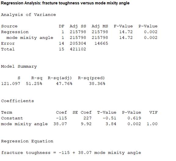
From the MINITAB output, the regression line is
Thus, the regression line for the variables fracture toughness
Interpretation:
The slope estimate implies an increase in fracture toughness by 38.07
The test hypotheses are given below:
Null hypothesis:
That is, there is no useful relationship between the variables fracture toughness
Alternative hypothesis:
That is, there is useful relationship between the variables fracture toughness
T-test statistic:
The test statistic is,
From the MINITAB output, the test statistic is 3.84 and the P-value is 0.002.
Thus, the value of test statistic is 3.84 and P-value is 0.002.
Level of significance:
Here, level of significance is not given.
So, the prior level of significance
Decision rule based on p-value:
If
If
Conclusion:
The P-value is 0.002 and
Here, P-value is less than the
That is
By the rejection rule, reject the null hypothesis.
Thus, there is enough evidence to conclude that the predictor variable mode-mixity angle is useful for predicting the value of the response variable fracture toughness.
b.
Test whether there is enough evidence to conclude that the change in fracture toughness associated with 1 degree increase in mode-mixity angle is greater than 50
b.
Answer to Problem 76SE
There is no sufficient evidence to conclude that the change in fracture toughness associated with 1 degree increase in mode-mixity angle is greater than 50
Explanation of Solution
Calculation:
From the MINITAB output obtained in part (a), the slope coefficient of the regression equation is
Here,
Claim:
Here, the claim is that the true average change in the fracture toughness associated with 1 degree increase in mode-mixity angle is greater than 50
The test hypotheses are given below:
Null hypothesis:
That is, the average change in the fracture toughness associated with 1 degree increase in mode-mixity angle is less than or equal to 50
Alternative hypothesis:
That is, the average change in the fracture toughness associated with 1 degree increase in mode-mixity angle is greater than 50
Test statistic:
The test statistic is,
Degrees of freedom:
The number of concrete beams that are sampled is
The degrees of freedom is,
Thus, the degree of freedom is 14.
Level of significance:
Here, level of significance is not given.
So, the prior level of significance
Critical value:
Software procedure:
Step by step procedure to obtain the critical value using the MINITAB software:
- Choose Graph > Probability Distribution Plot choose View Probability > OK.
- From Distribution, choose ‘t’ distribution and enter 14 as degrees of freedom.
- Click the Shaded Area tab.
- Choose Probability Value and Right Tail for the region of the curve to shade.
- Enter the Probability value as 0.05.
- Click OK.
Output using the MINITAB software is given below:
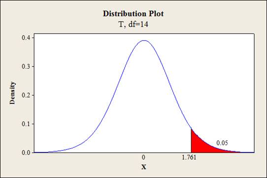
From the output, the critical value is 1.761.
Thus, the critical value is
From the MINITAB output obtained in part (a), the estimate of error standard deviation of slope coefficient is
Test statistic under null hypothesis:
Under the null hypothesis, the test statistic is obtained as follows:
Thus, the test statistic is -1.2026.
Decision criteria for the classical approach:
If
Conclusion:
Here, the test statistic is -1.2026 and critical value is 1.761.
The t statistic is less than the critical value.
That is,
Thus, the decision rule is, failed to reject the null hypothesis.
Hence, the average change in the fracture toughness associated with 1 degree increase in mode-mixity angle is less than or equal to 50
Therefore, there is no sufficient evidence to conclude that the change in fracture toughness associated with 1 degree increase in mode-mixity angle is greater than 50
c.
Explain whether the new observations of the variable mode-mixity angle give more precise estimate of slope coefficient than the actual observations.
c.
Answer to Problem 76SE
No, the new observations of the variable mode-mixity angle do not give more precise estimate of slope coefficient than the actual observations.
Explanation of Solution
Given info:
The data represents the new values of the variable mode-mixity angle, at which the response variable fracture toughness is predicted.
Calculation:
Confidence interval:
The general formula for the confidence interval for the slope of the regression line is,
Where,
The precision of the confidence interval increases with the decrease in the error standard deviation of the slope.
That is, the precision will be high for lower value of
Error sum of square: (SSE)
The variation in the observed values of the response variable that is not explained by the regression is defined as the regression sum of squares. The formula for error sum of square is
Estimate of error standard deviation of slope coefficient:
The general formula for the estimate of error standard deviation of slope coefficient is,
The defining formula for
Here, the estimate of error standard deviation of slope coefficient depends on the value of
The estimate of error standard deviation of slope coefficient decreases with the increase in the value of
The margin of error is product of critical value and standard error of the statistic. The higher width of the confidence interval indicates larger standard error of statistic. Hence, the margin of error also increases.
Therefore, the width of the confidence interval decreases with the decrease in value of error standard deviation. In other words it can be said that the precision decreases with the decrease in the value of
The value of
| 1 | 16.52 | 272.9104 |
| 2 | 17.53 | 307.3009 |
| 3 | 18.05 | 325.8025 |
| 4 | 18.05 | 325.8025 |
| 5 | 22.39 | 501.3121 |
| 6 | 23.89 | 570.7321 |
| 7 | 25.50 | 650.25 |
| 8 | 24.89 | 619.5121 |
| 9 | 23.48 | 551.3104 |
| 10 | 24.98 | 624.0004 |
| 11 | 25.55 | 652.8025 |
| 12 | 25.90 | 670.81 |
| 13 | 22.65 | 513.0225 |
| 14 | 23.69 | 561.2161 |
| 15 | 24.15 | 583.2225 |
| 16 | 24.45 | 597.8025 |
| Total |
Here,
Thus, the value of
Hence, the covariance is
The value of
| 1 | 16 | 256 |
| 2 | 16 | 256 |
| 3 | 18 | 324 |
| 4 | 18 | 324 |
| 5 | 20 | 400 |
| 6 | 20 | 400 |
| 7 | 20 | 400 |
| 8 | 20 | 400 |
| 9 | 22 | 484 |
| 10 | 22 | 484 |
| 11 | 22 | 484 |
| 12 | 22 | 484 |
| 13 | 24 | 576 |
| 14 | 24 | 576 |
| 15 | 26 | 676 |
| 16 | 26 | 676 |
| Total |
Here,
Thus, the value of
Hence, the covariance is
The value of
That is,
Hence, the estimate of error standard deviation of slope coefficient is lower for old observations.
Therefore, the precision is high for old observations.
Thus, the new observations of the variable mode-mixity angle do not give more precise estimate of slope coefficient than the actual observations.
d.
Find the
Find the prediction interval of fracture toughness for a single sandwich panel of 18 degrees mode-mixity angle.
Find the interval estimate for the true mean fracture toughness of all sandwich panels with 22 degrees mode-mixity angle.
Find the prediction interval of fracture toughness for a single sandwich panel of 22 degrees mode-mixity angle.
d.
Answer to Problem 76SE
The 95% specified confidence interval for the true mean fracture toughness of all sandwich panels with 18 degrees mode-mixity angle is
The 95% prediction interval of fracture toughness for a single sandwich panel with 18 degrees mode-mixity angle is
The 95% specified confidence interval for the true mean fracture toughness of all sandwich panels with 22 degrees mode-mixity angle is
The 95% prediction interval of fracture toughness for a single sandwich panel with 22 degrees mode-mixity angle is
Explanation of Solution
Calculation:
Here, the regression equation is
Expected fracture toughness when the mode-mixity angle is 18 degrees:
The expected fracture toughness with 18 degrees mode-mixity angle is obtained as follows:
Thus, the expected fracture toughness with 18 degrees mode-mixity angle is 570.26.
95% confidence interval of true mean fracture tough for an angle of 18 degrees:
The general formula for the
Where,
From the MINITAB output in part (a), the value of the standard error of the estimate is
The value of
| 1 | 16.52 | 272.9104 |
| 2 | 17.53 | 307.3009 |
| 3 | 18.05 | 325.8025 |
| 4 | 18.05 | 325.8025 |
| 5 | 22.39 | 501.3121 |
| 6 | 23.89 | 570.7321 |
| 7 | 25.50 | 650.25 |
| 8 | 24.89 | 619.5121 |
| 9 | 23.48 | 551.3104 |
| 10 | 24.98 | 624.0004 |
| 11 | 25.55 | 652.8025 |
| 12 | 25.90 | 670.81 |
| 13 | 22.65 | 513.0225 |
| 14 | 23.69 | 561.2161 |
| 15 | 24.15 | 583.2225 |
| 16 | 24.45 | 597.8025 |
| Total |
Here,
The mean mode-mixity angle is,
Thus, the mean mode-mixity angle is
Covariance term
Thus, the value of
Hence, the covariance is
Since, the level of confidence is not specified. The prior confidence level 95% can be used.
Critical value:
For 95% confidence level,
Degrees of freedom:
The sample size is
The degrees of freedom is,
From Table A.5 of the t-distribution in Appendix A, the critical value corresponding to the right tail area 0.025 and 14 degrees of freedom is 2.145.
Thus, the critical value is
The 95% confidence interval is,
Thus, the 95% specified confidence interval for the true mean fracture toughness of all sandwich panels with 18 degrees mode-mixity angle is
Interpretation:
There is 95% confident that, the true mean fracture toughness of all sandwich panels with 18 degrees mode-mixity angle lies between 453.6507 and 686.8693.
95% prediction interval of fracture tough for an angle of 18 degrees:
Prediction interval for a single future value:
Prediction interval is used to predict a single value of the focus variable that is to be observed at some future time. In other words it can be said that the prediction interval gives a single future value rather than estimating the mean value of the variable.
The general formula for
where
The 95% prediction interval is,
Thus, the 95% prediction interval of fracture toughness for a single sandwich panel with 18 degrees mode-mixity angle is
Interpretation:
For repeated samples, there is 95% confident that the fracture toughness for a single sandwich panel with 18 degrees mode-mixity angle lies between 285.5331 and 854.9569.
Expected fracture toughness when the mode-mixity angle is 22 degrees:
The expected fracture toughness with 22 degrees mode-mixity angle is obtained as follows:
Thus, the expected fracture toughness with 22 degrees mode-mixity angle is 722.54.
95% confidence interval of true mean fracture tough for an angle of 22 degrees:
The 95% confidence interval is,
Thus, the 95% specified confidence interval for the true mean fracture toughness of all sandwich panels with 22 degrees mode-mixity angle is
Interpretation:
There is 95% confident that, the true mean fracture toughness of all sandwich panels with 22 degrees mode-mixity angle lies between 656.3689 and 788.7111.
95% prediction interval of fracture tough for an angle of 22 degrees:
The 95% prediction interval is,
Thus, the 95% prediction interval of fracture toughness for a single sandwich panel with 22 degrees mode-mixity angle is
Interpretation:
For repeated samples, there is 95% confident that the fracture toughness for a single sandwich panel with 22 degrees mode-mixity angle lies between 454.491 and 990.589.
Want to see more full solutions like this?
Chapter 12 Solutions
EBK PROBABILITY AND STATISTICS FOR ENGI


- A study of the properties of metal plate-connected trusses used for roof support yielded the following observations on axial stiffness index (kips/in.) for plate lengths 4, 6, 8, 10, and 12 in: 4: 323.2 409.5 311.0 326.5 316.8 349.8 309.7 6: 423.1 347.2 361.0 404.5 331.0 348.9 381.7 8: 393.4 366.2 351.0 357.1 409.9 367.3 382.0 10: 362.7 452.9 461.4 433.1 410.6 384.2 362.6 12: 418.4 441.8 419.9 410.7 473.4 441.2 465.8 Does variation in plate length have any effect on true average axial stiffness? State the relevant hypotheses using analysis of variance. H0: ?1 ≠ ?2 ≠ ?3 ≠ ?4 ≠ ?5Ha: at least two ?i's are equalH0: ?1 = ?2 = ?3 = ?4 = ?5Ha: all five ?i's are unequal H0: ?1 = ?2 = ?3 = ?4 = ?5Ha: at least two ?i's are unequalH0: ?1 ≠ ?2 ≠ ?3 ≠ ?4 ≠ ?5Ha: all five ?i's are equal Test the relevant hypotheses using analysis of variance with ? = 0.01. Display your results in an ANOVA table. (Round your answers to two decimal places.) Source Degrees offreedom Sum…arrow_forwardThe article "Effect of Microstructure and Weathering on the Strength Anisotropy of Porous Rhyolite" (Y. Matsukura, K. Hashizume, and C. Oguchi, Engineering Geology, 2002:39- 17) investigates the relationship between the angle betwween cleavage and flow structure and the strength of porous rhyolite. Strengths (in MPa) were measured for a mumber of specimens cut at various angles. The mean and standard deviation of the strengths for each angle are presented in the following table. Angle Mean 0° 22.9 Sample Size Standard Deviation 2.98 12 15° 22.9 1.16 30° 19.7 3.00 45° 14.9 2.99 60° 13.5 2.33 75° 11.9 2.10 90 14.3 3.95 6. Can you conclude that strength varies with the angle?arrow_forwardA study was carried out to compare the writing lifetimes of four premium brands of pens. It was thought that the writing surface might affect life- time, so three different surfaces were randomly se- tected. A writing machine was used to ensure that conditions were otherwise homogeneous (e.g., con- stant pressure and a fixed angle). The accompany- ing table shows the two lifetimes (min) obtained for each brand-surface combination. In addition, EEEr = 11,499,492 and EExj, = 22,982,552, Writing Surface 1 2 3 1 709, 659 713, 726 660, 643 Brand 2 668, 685 722, 740 692, 720 of Pen 3 659, 685 666, 684 678, 750 4 698, 650 704, 666 686, 733 4112 4227 4122 4137 5413 5621 5564 16,598 Carry out an appropriate ANOVA, and state your conclusions.arrow_forward
- A study of the properties of metal plate-connected trusses used for roof support yielded the following observations on axial stiffness index (kips/in.) for plate lengths 4, 6, 8, 10, and 12 in: 4: 333.2 409.5 311.0 326.5 316.8 349.8 309.7 6: 433.1 347.2 361.0 404.5 331.0 348.9 381.7 8: 382.4 366.2 351.0 357.1 409.9 367.3 382.0 10: 350.7 452.9 461.4 433.1 410.6 384.2 362.6 12: 413.4 441.8 419.9 410.7 473.4 441.2 465.8 LUSE SALT Does variation in plate length have any effect on true average axial stiffness? State the relevant hypotheses using analysis of variance. O Hoi Hy #fly #Hz" Ha #Hs H: all five μ's are equal O Hoi H₂H₂ = H3 = HaHs H: at least two μ's are unequal O Hoi H₂ = H₂ = H₂ "HaHs H: all five μ's are unequal O Hoi H₂ #4₂ # Hz*H4 *H5 H: at least two μ's are equal Test the relevant hypotheses using analysis of variance with a = 0.01. Display your results in an ANOVA table. (Round your answers to two decimal places.) Degrees of Sum of Mean freedom Squares Squares Error Total…arrow_forwardRecently there has been increased use of stainless steel claddings in industrial settings. Claddings are used to finish the exterior walls of a building and help weatherproof the structure. To ensure the quality of claddings, it is essential to know how welding parameters impact the cladding process. The authors of “Mathematical Modeling of Weld Bead Geometry, Quality, and Productivity for Stainless Steel Claddings Deposited by FCAW” (J. Mater. Engr. Perform., 2012: 1862–1872) in vestigated how y 5 deposition rate was influenced by x1 = feed rate (Wf , in m/min) and x2 = welding speed (S, in cm/min). The following 22 observations correspond to the experiment condition where applied voltage was less than 30v: y: 2.718 3.881 2.773 3.924 2.740 3.870 x1 : 17.0 10.0 7.0 10.0 7.0 10.0 x 2 : 30 30 50 50 30 30 y: 2.847 3.901 2.204 4.454 3.324 3.319 x1 : 7.0 10.0 5.5 11.5 8.5 8.5 x2 : 50 50 40 40 40 20 The whole data and Question parts are attachedarrow_forwardComputer chips often contain surface imperfections.For a certain type of computer chip, theprobability mass function of the number of defects X is presented in the following table.arrow_forward
- Eyeglassomatic manufactures eyeglasses for different retailers. They test to see how many defective lenses they made in a time period. Table #4.2.2 gives the defect and the number of defects. Table #4.2.2: Number of Defective Lenses Defect type Number of defects Scratch 5865 Right shaped – small 4613 Flaked 1992 Wrong axis 1838 Chamfer wrong 1596 Crazing, cracks 1546 Wrong shape 1485 Wrong PD 1398 Spots and bubbles 1371 Wrong height 1130 Right shape – big 1105 Lost in lab 976 Spots/bubble – intern 976 Find the probability of picking a lens that is scratched or flaked. Find the probability of picking a lens that is the wrong PD or was lost in lab. Find the probability of picking a lens that is not scratched. Find the probability of picking a lens that is not the wrong shape.arrow_forward2. A city's transportation committee has conducted research on traffic and car accidents for downtown streets. There is a 9% chance of being involved in a car accident when 15 or more cars are driving on Johnson Street and a 7.5% chance when 20 or more cars are driving on Dublin Street. The two streets intersect to form a risk area with a radius of 0.1 mi. Approximate the density of cars per square mile in the risk area when 17 cars are on Johnson Street and 21 cars are on Dublin Street. Use 3.14 for TT. There are approximately 1,082 cars per square mile in the risk area. There are approximately 2,674 cars per square mile in the risk area. There are approximately 2,165 cars per square mile in the risk area. There are approximately 1,210 cars per square mile in the risk area.arrow_forward.... At wind speeds above 1000 centimeters per second (cm/sec), significant sand-moving events begin to occur. Wind speeds below 1000 cm/sec deposit sand and wind speeds above 1000 cm/sec move sand to new locations. The cyclic nature of wind and moving sand determines the shape and location of large dunes. At a test site, the prevailing direction of the wind did not change noticeably. However, the velocity did change. Sixty-two wind speed readings gave an average velocity of x = 1075 cm/sec. Based on long-term experience, o can be assurhed to be 250 cm/sec. (a) Find a 95% confidence interval for the population mean wind speed at this site. (Round your answers to the nearest whole number.) lower limit cm/sec upper limit cm/sec (b) Does the confidence interval indicate that the population mean wind speed is such that the sand is always moving at this site? Explain. O No. This interval Indicates that the population mean wind speed is such that the sand may not always be moving at this…arrow_forward
- The following are the weight losses of certain machine parts due to friction (in milligrams) when used with three different lubricants: Lubricant 1: 13 11 10 13 Lubricant 2: 9. 11 Lubricant 3: 7 6. Test at the 0,01 level of significance whether the type of lubricant effects the weight loss of the machine parts due to friction. While carrying out the test, follow the steps below and answer the questions. 1- Determine the null and alternative hypotheses. Ho: H: 2-Fill in the following ANOVA Table. ANOVA Table Source of Variation Degrees of Freedom Sum of Squares Mean Sum of Squares Treatment Error Total 3-State your decision and conclusion.arrow_forwardSuppose you fit the first-order model y = Po + B, x, + B2x2 + B3X3 + B,x4 + B5X5 + ɛ to n=28 data points and obtain SSE = 0.33 and R = 0.94. Complete parts a and b. a. Do the values of SSE and R suggest that the model provides a good fit to the data? Explain. A. Yes. Since R = 0.94 is close to 1, this indicates the model provides a good fit. Also, SSE = 0.33 is fairly small, which indicates the model provides a good fit. B. There is not enough information to decide. No. Since R = 0.94 is close to 1, this indicates the model does not provide a good fit. Also, SSE = 0.33 is fairly small, which indicates the model does not provide a good fit. b. Is the model of any use in predicting Test the null hypothesis Ho: B, = B2 = ... = B5 = 0 against the alternative hypothesis: At least of the %3D parameters B1, B2, B5 is nonzero. Use a = 0.05. The test statistic is (Round to two decimal places as needed.)arrow_forwardA researcher wants to identify the average number of hours spent by senior high school students playing online games per day. From a sample of 100 senior high students, an average of 6 hours was determined. What is the parameter? O a. average number of hours spent by senior high school students playing online games per day Ob. a sample of 100 senior high students Oc. an average of 6 hours Od. all senior high school studentsarrow_forward
 MATLAB: An Introduction with ApplicationsStatisticsISBN:9781119256830Author:Amos GilatPublisher:John Wiley & Sons Inc
 Probability and Statistics for Engineering and th...StatisticsISBN:9781305251809Author:Jay L. DevorePublisher:Cengage Learning
 Statistics for The Behavioral Sciences (MindTap C...StatisticsISBN:9781305504912Author:Frederick J Gravetter, Larry B. WallnauPublisher:Cengage Learning
 Elementary Statistics: Picturing the World (7th E...StatisticsISBN:9780134683416Author:Ron Larson, Betsy FarberPublisher:PEARSON
 The Basic Practice of StatisticsStatisticsISBN:9781319042578Author:David S. Moore, William I. Notz, Michael A. FlignerPublisher:W. H. Freeman
 Introduction to the Practice of StatisticsStatisticsISBN:9781319013387Author:David S. Moore, George P. McCabe, Bruce A. CraigPublisher:W. H. Freeman