
(a)
The aggregate
(a)
Explanation of Solution
Figure 1 shows the aggregate demand and
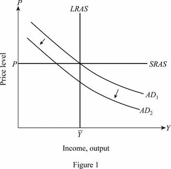
The horizontal axis of Figure 1 measures the income and output, and the vertical axis measures the price level. The aggregate demand curve, AD1, is the initial aggregate demand curve. The horizontal curve SRAS parallel to the output axis is the short-run supply curve, and the vertical curve LRAS is the long run
Here, M is the money supply, V is the velocity of money, P is the price level, and Y is the output. This relationship clearly points that a decrease in the money supply would lead to a proportionate decrease in the nominal output. Thus, when the value of velocity of money is given for a particular level of output, a reduction in the money supply would lead to a reduction in the price level.
Quantity theory of money: Quantity theory of money refers to the relationship between the price level and money supply. The quantity theory of money equation is
(b)
The change in output and price levels.
(b)
Explanation of Solution
Figure 2 shows the aggregate demand and aggregate supply curves in the long run.
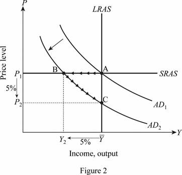
The horizontal axis of Figure 2 measures the income and output, and the vertical axis measures the price level. The aggregate demand curve, AD1, is the initial aggregate demand curve. The horizontal curve SRAS parallel to the output axis is the short-run supply curve, and the vertical curve LRAS is the long-run aggregate supply curve. It is known that the price level is fixed in the short run, which is indicated by the horizontal aggregate supply curve. When the money supply reduces, the aggregate demand curve shifts from AD1 to AD2, leading to a movement from point A to point B. This movement implies that the level of output reduces, while the price remains constant. However, in the long run, the prices are also variable, and hence the price reduces, and the economy restores full employment at the point C.
It is known that quantity theory of money is given by Equation (1) as follows:
Let one assume that the velocity is constant, and the percentage reduction in money supply is 5%.
The quantity equation can be expressed in percentage terms using Equation (2) as follows:
In the short run, the price level is constant; thus, the change in price level is zero, and the change in velocity is also 0. Substituting the respective values in Equation (2), the percentage change in output can be calculated as follows:
Thus, the percentage change in the level of output is equal to the percentage change in the money supply, which is 5%.
Thus, a 5 % reduction in the money supply leads to a 5 % reduction in the quantity of output in the short run.
In the long run, the output level is restored as the price level is flexible. Thus, the change in output in the long run is zero. The change in the price level in the long run can be calculated as follows:
Thus, a 5% reduction in the money supply would lead to a 5% reduction in the price level in the long run.
Quantity theory of money: Quantity theory of money refers to the relationship between the price level and money supply. The quantity theory of money equation is
(c)
The level of
(c)
Explanation of Solution
It is known that Okun’s law is the mathematical relationship between unemployment and real GDP in the long run. When the rate of unemployment is u and the rate of output is Y, the Okun’s law is approximated using Equation (3) as follows:
In the short run, the reduction in the level of output reduces the rate of employment, and hence, the rate of unemployment increases. It is known that the output reduces by 55 in the short run. The rate of unemployemnt can be calculated by substituting the respective values in Equation (3) as follows:
Thus, a 5% reduction in the output in the short run leads to an increase in the rate of unemployment by 4%. However, in the long run, the level of output and employment is restored, and hence the rate of unemployment in the long run remains unchanged.
Unemployment rate: Unemployment rate refers to the percentage of unemployed people in the labor force. Unemployment is a state that occurs in an economy when the able and willing persons cannot find any work or job. But, these people are keenly seeking for jobs.
(d)
The rate of interest.
(d)
Explanation of Solution
Figure 3 shows the changes in the interest rate.
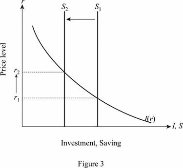
The horizontal axis of Figure 3 measures the investment and saving, and the vertical axis measures the real interest rate. The downward doping curve I indicates the interest rate.
The vertical curve S1 is the initial money supply curve. It is known that the savings is the difference between the total income and consumption. If the national savings are concerned, it is the difference between the total income, consumption, and the Government expenditure. A reduction in the total income would lead to a reduction in the national savings. This implies that the money supply reduces from S1 to S2. The reduction in the supply of money leads to an increase in the rate of interest from r1 to r2. In the long run, since the level of output is restored, the interest rate also falls back to r1.
Short run: Short run is defined as the period in which production can be increased only by varying one of the input factors, and the others remain fixed.
Long run: Long run is defined as the period in which production can be increased by changing all the input factors.
Savings: Saving is a portion of disposable income that is left over after consumption. National savings include private savings and government savings.
Want to see more full solutions like this?

- In the figure at right, assume the economy starts out in equilibrium at point d. If the Fed increases the money supply so that the new aggregate demand curve is AD3, then the new short-run equilibrium will be at point A. i. O B. c. C. b. D. a. Price Level 130 120 100 e b LRAS 9 с SRAS₁ SRAS₂ AD₁ Real GDP per Year ($ trillions) SRAS3 AD3 AD₂arrow_forwardIf money supply rises, will the price level rise by the same percentage? It all depends on what happens to V and Y. The effects will tend to differ in the short run from the long run. Delete the wrong words in the following statements: (a) In the short run, V can change substantially / is unlikely to change much at all when money supply changes. (b) In the short run, a rise in MV (i.e. a rise in aggregate demand) will lead to a rise in the price level / may or may not lead to a rise in the price level depending on the degree of slack in the economy.arrow_forwardIn the following table, determine how each event affects the position of the long-run aggregate supply (LRAS) curve. Direction of LRAS Curve Shift Many workers leave to pursue more lucrative careers in foreign economies. A scientific breakthrough significantly increases food production per acre of farmland. A natural disaster destroys a significant amount of the economy's production facilities.arrow_forward
- Suppose that the money supply increases by 20 percent. If there is no inflation, what does the quantity theory of money tell us must happen to real GDP? (Assume that the velocity of money is constant.) Select an answer and submit. For keyboard navigation, use the up/down arrow keys to select an answer. a It must increase by more than 20% It must increase by less than 20% C It stays the same d. It must increase by 20%arrow_forwardA nation's economy is in short run equilibrium. The actual unemployment rate is lower than the natural rate of unemployment. A. Show each of the following using a correctly labeled graph of the long run aggregate supply curve, short run aggregate supply curve, and aggregate demand curve: i. Current price level, labeled PL1, and current output level, labeled Y1 ii. The full employment output level, labeled Yf. B. Use a correctly labeled money market graph to show how the country's central bank action can move the economy toward its long run equilibrium. Indicate how this affects the equilibrium nominal interest rate in the short run. incarrow_forwardSuppose that government decides to support the firms for their investments in research and the development.Assuming this support increases productivity in the economy, use aggregate demand and supply analysis to predict the short-run and long-run effects on inflation and output. Show these effects on a graph and explainthe results in detail.arrow_forward
- Assume that a country's economy is in short-run equilibrium and the actual unemployment rate is lower than the natural rate of unemployment. A. Using a correctly labeled graph of the long-run aggregate supply curve, short-run aggregate supply curve, and aggregate demand curve, show each of the following: i. Current price level, labeled P1, and current output level, labeled Y1 ii. The full employment output level, labeled Yf B. What open market operation can the country's central bank use to move the economy toward its long run equilibrium? C. Use a correctly labeled money market graph to show how the country's central bank action to move the economy toward its long-run equilibrium affects the equilibrium nominal interest rate in the short run. D. Based on the interest rate change from Part C, will each of the following increase, decrease, or remain the same in the short run? i. Real output. Explain. ii. Natural rate of unemployment E. Assume instead that…arrow_forwardExplain how an increase in a price level will affect the demand for money and the aggregate demand. Use relevant graphs to support your answer.arrow_forwardA.W. Phillips concluded that there is a trade-off between the inflation rate and the unemployment rate in the short-run. The graph to the right can be used to show the relationship between those two variables. 10- Using the 3-point curved line drawing tool, draw the relationship that A. W. Phillips saw between the unemployment and inflation rates in the graph to the right. Label the curve 'PC'. 8- Carefully follow the instructions above, and only draw the required objects. 6- However, the U.S. experience shows that there is no clear relationship between the unemployment rate and the inflation rate. Since the 1950s data indicate that changes in the inflation rate have not altered the unemployment rate. Thus, empirical data provide evidence that the long run Phillips Curve is 2- 0- 10 12 14 16 18 20 -2- -4- -6- Unemplovment Rate Inflation Rate 4.arrow_forward
- Suppose the Fed doubles the growth rate of the quantity of money in the economy. In the long run, the increase in money growth will change which of the following? Check all that apply. The inflation rate C The price level C The level of technological knowledge The size of the labor force Suppose the economy produces real GDP of $70 billion when unemployment is at its natural rate. Use the purple points (diamond symbol) to plot the economy's long-run aggregate supply (LRAS) curve on the graph. 132 128 LRAS 124 120 116 112 108 104 100 10 20 30 40 50 60 70 80 OUTPUT (Billions of dollars) Suppose the government passes a law that significantly increases the minimum wage. The policy will cause the natural rate of unemployment to which will: O Shift the long-run aggregate supply curve to the right O Shift the long-run aggregate supply curve to the left O Not affect the long-run aggregate supply curve PRICE LEVELarrow_forwardProblem Solving T 1. Suppose the Central Bank reduces the money supply by 5 percent. Assume the velocity of money is constant. a. What happens to the aggregate demand curve? b. What happens to the level of output and the price level in the short run and in the long run? Give a precise numerical answer. C. What happens to the real interest rate in the short run and in the long run? Here, your answer should just give the direction of the changes.arrow_forward3)Show and explain the effects of an increase in aggregate demand in the long-run and short-run by using AD–AScurves.2)Show and explain by using a graph, what will happen to the price level and real GDP if the quantity of moneyincreases and the increase is not anticipated; that is, the price level is not expected to change.1)By using aggregate demand (AD) and aggregate supply (AS) curves, show and explain the effects of ananticipated increase in money supply on macroeconomic equilibrium according to Rational ExpectationsHypothesis.arrow_forward
 Exploring EconomicsEconomicsISBN:9781544336329Author:Robert L. SextonPublisher:SAGE Publications, Inc
 Economics (MindTap Course List)EconomicsISBN:9781337617383Author:Roger A. ArnoldPublisher:Cengage Learning