Answered: 50 Weighted CO2 Emmisions 50 Diesel…

Refrigeration and Air Conditioning Technology (MindTap Course List)

8th Edition

ISBN:9781305578296

Author:John Tomczyk, Eugene Silberstein, Bill Whitman, Bill Johnson

Publisher:John Tomczyk, Eugene Silberstein, Bill Whitman, Bill Johnson

Chapter31: Gas Heat

Section: Chapter Questions

Problem 5RQ: The specific gravity of natural gas is A. 0.08. B. 1.00. C. 0.42. D. 0.60.

See similar textbooks

Related questions

Question

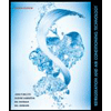
I’m making the graph that you see in the picture but the code that I’m using makes the line with to many curves. Could you make the lines look like the one that you see on the graph. Don’t change the color just make it with a little bit less curves like you see in the picture. Use this code on MATLAB and fix it. % Sample data for Diesel and Petrol cars carPosition = linspace(1, 60, 50); % Assumed positions of cars % Fix the random seed for reproducibility rng(50); % Assumed CO2 emissions for Diesel and Petrol CO2Diesel = 25 + 5*cos(carPosition/60*2*pi) + randn(1, 50)*5; % Random data for Diesel CO2Petrol = 20 + 5*sin(carPosition/60*2*pi) + randn(1, 50)*5; % Random data for Petrol % Fit polynomial curves pDiesel = polyfit(carPosition, CO2Diesel, 3); pPetrol = polyfit(carPosition, CO2Petrol, 3); % Generate points for best fit lines fitDiesel = polyval(pDiesel, carPosition); fitPetrol = polyval(pPetrol, carPosition); % Combined best fit combinedFit = (fitDiesel + fitPetrol) / 2; % Plotting the data figure; hold on; % Define the split index and shorten the purple line splitIndex = round(length(carPosition) / 2); shortenIndex = round(length(carPosition) * 0.8); % Plot the combined best fit line (connect orange and purple, purple line shorter) plot(carPosition(1:shortenIndex), combinedFit(1:shortenIndex), 'Color', [1, 0.5, 0], 'LineWidth', 2); % Orange to shorter purple plot(carPosition(shortenIndex:end), combinedFit(shortenIndex:end), 'Color', [0.5, 0, 1], 'LineWidth', 2); % Shortened Purple % Petrol data scatter(carPosition, CO2Petrol, 'o', 'MarkerEdgeColor', [0 0.5 1]); % Blue for Petrol % Diesel data scatter(carPosition, CO2Diesel, 'o', 'MarkerEdgeColor', [1 0.5 0]); % Orange for Diesel % Customize the plot xlabel('Car Position'); ylabel('CO2 Weighted Percentage'); title('Weighted CO2 Emissions'); % Adjust axis limits xlim([1 60]); ylim([15 35]); % Add a legend with custom names legend('Combined Best Fit - Orange', 'Combined Best Fit - Purple', 'Petrol', 'Diesel'); % Add grid lines grid on; hold off;

50
Weighted CO2 Emmisions
50
Diesel
Petrol
10
40
30
CO2 Weighted Percentage
20
8
10
0
о
о
800
0 0
о
%
-10
0
୦୧
о
10
10
20
30
40
40
50
60
Car Position
Diesel Best Fit
Petrol Best Fit

Expert Solution

Step by step

Solved in 2 steps with 1 images

SEE SOLUTION Check out a sample Q&A here

50 Weighted CO2 Emmisions 50 Diesel Petrol 10 40 30 CO2 Weighted Percentage 20 8 10 0 о о 800 0 0 о % -10 0 ୦୧ о 10 10 20 30 40 40 50 60 Car Position Diesel Best Fit Petrol Best Fit